Tuesday, January 16, 2024

Heart Disease Prediction – Application of Scikit-Learn and Machine Learning

We all know that the cardiovascular diseases (CVDs), heart disease, acknowledged as the most common cause of death during the preceding several decades, is now recognized as the most lethal condition, not just in India but throughout the globe. In humans, the heart is important. A small error can result in tiredness issues or even death. One of the most significant challenges confronting medical sector today is the prediction or forecasting of heart illness. It is associated with numerous and intimidating factors and components. An early diagnosis must be made using a prediction model that is reliable, trustworthy, and reasonable in order to achieve rapid disease treatment. It has been discovered that Machine Learning and Deep Learning may help with decision-making and prediction-making using the vast amounts of data that gathered from several healthcare firms. Machine learning methods and approaches have been used to automate the study of big and complicated medical information. Recently, some of the decorated researchers have employed various machine learning to assist the healthcare sectors and professionals to identify heart- related illness.

Before implementing the machine learning models, we need authenticated medical records such as tabular data to predict the heart related illnesses. Let’s look at the data in hand which is taken from the open-source platform know as Kaggle, and this is the link to Heart Disease Dataset (kaggle.com). This data contains the following attributes.

Dataset Attributes

Exploratory Data Analysis

What is Exploratory Data Analysis?

Exploratory Data Analysis (EDA) is an essential stage in the data analysis process that entails analyzing and graphically representing data sets to comprehend their primary attributes, reveal patterns, spot anomalies, and ascertain connections between variables. The main objective of Exploratory Data Analysis (EDA) is to get a deep understanding of the fundamental organization of the data, formulate hypotheses, and provide guidance for the later stages of analysis or modeling.

Let's open the CSV (Comma Separated Values) file, to get the Heart Disease Detection dataset. For the presented context, I will be using python programming language for code example.

1. Importing the important libraries for exploratory data analysis

import numpy as np 

import pandas as pd

import matplotlib.pyplot as plt

import seaborn as sns

import warnings

warnings.filterwarnings("ignore")

2. Importing the dataset

df = pd.read_csv("/kaggle/input/heart-disease-dataset/heart.csv")
df.head() # viewing the first five rows of the dataset


Let's look at the shape of the dataset.
df.shape
From the shape of the dataset, we can observe that the dataset contains total 1025 data rows and 14 columns or attributes.  Let's look at the data types of the different attributes of the data.
df.info()

Almost every attribute of the dataset has integer values except oldpeak is of float type. Let's look at the different properties of the dataset such as mean, min, standard deviation and more...
df.describe().T

3. Exploratory Data Analysis (EDA)

Let's look at the Gender distribution of the dataset. Where 1 - Male and 0 - Female.
df['sex'].value_counts()

In the given dataset there are total 713 male records and 312 female records.  Let's create the bar chart for the same.
df['sex'].value_counts().plot(kind='bar', color=['orange', 'green'])

Let's look at the target values in the dataset. Where target: 1- Positive and 0 - Negative.
df['target'].value_counts()

In the dataset there are total 526 positive records and 499 negative records. Let's create the bar chart for the same.
df['target'].value_counts().plot(kind='bar', color=['red', 'green'])

Let's look at how many males and females in the records have heart diseases.
pd.crosstab(df.target, df.sex)

fig = sns.countplot(x = 'target', data = df, hue = 'sex')
fig.set_xticklabels(labels=["Doesn't have heart disease", 'Has heart disease'], rotation=0)
plt.legend(['Female', 'Male'])
plt.title("Heart Disease Frequency for Sex");

4. Checking the Correlation Within Dataset Attributes

x = df.corr()
plt.figure(figsize = (15,8))
sns.heatmap(x,annot = True)

From heatmap we can clearly observe that no column is shown significant contribution among all the attributes of the dataset. So, we are going to take all the features for the model evaluation. Let's look at the outliers among the dataset's attributes.
df.describe().T

The dataset columns `trestbps`, `chol`, `thalach` and `thal` shown some outliers among the datset.

5. Removing the Outliers from the Dataset

q1 = df['trestbps'].quantile(q = 0.25)
q3 = df["trestbps"].quantile(q = 0.75)
IQR = q3 - q1
IQR_lower_limit = int(q1 - (1.5*IQR))
IQR_upper_limit = int(q3 + (1.5*IQR))
print("Upper limit of IQR:",IQR_upper_limit)
print("Lower limit of IQR:",IQR_lower_limit)
cleaned_data = df[df["trestbps"]<IQR_upper_limit]

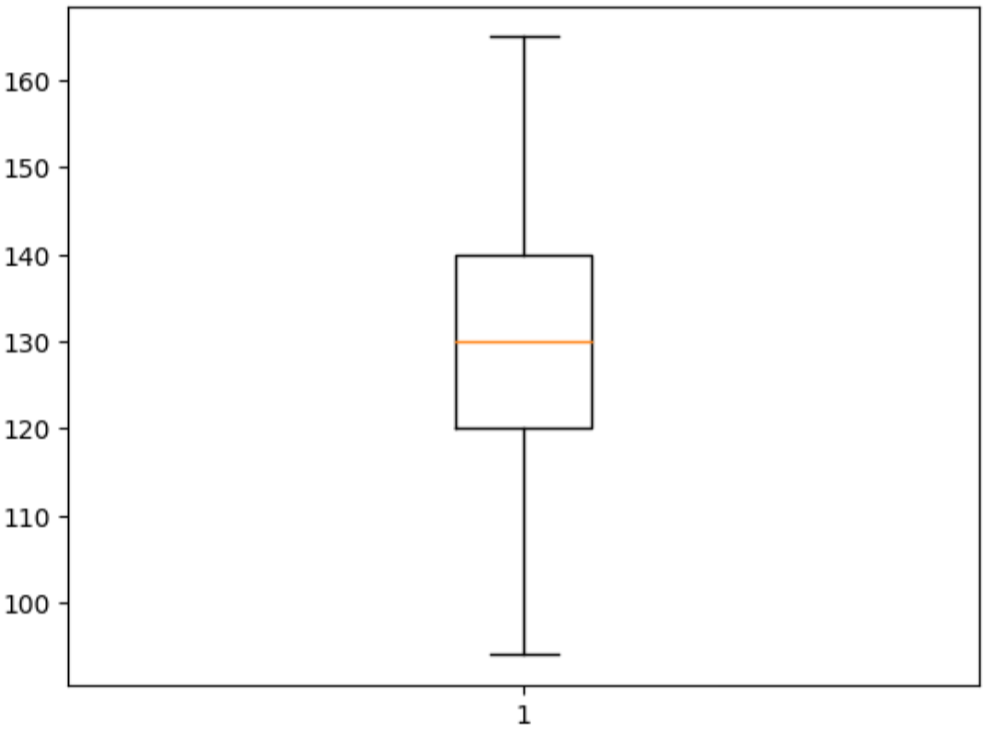
plt.boxplot(cleaned_data["trestbps"])
Now we can clearly see that there is no outlier in the dataset.
cleaned_data.shape

After removing the outliers there are only 980 records left in the dataset.

In this context we will employ the different methods of machine learning provided by the Scikit-Learn, to deploy such models that may help us predict the cardiovascular disease in timely manner to assist the healthcare system to aid the patient more effectively for more prompt recovery of patient. For this scenario we will implement machine learning models such as K-Nearest Neighbour (KNN), Logistic Regression (LR), and Random Forest (RF).

6. Building Model and Model Evaluation

6.1. One Hot-Encoding

cat_values = []
conti_values = []
for col in df.columns:
    if len(df[col].unique()) >= 10:
        conti_values.append(col)
    else:
        cat_values.append(col)
cat_values.remove('target')
cleaned_data = pd.get_dummies(cleaned_data, columns=cat_values)

6.2. Training and Testing Data Split

X = cleaned_data.drop(columns = 'target')
y = cleaned_data['target']
from sklearn.model_selection import train_test_split
X_train, X_test, y_train, y_test = train_test_split(X, y, test_size=0.20, random_state=1)

6.3. Importing Sklearn Libraries for Building Model and Model Evaluation

from sklearn import metrics
from sklearn.linear_model import LogisticRegression
from sklearn.neighbors import KNeighborsClassifier
from sklearn.ensemble import RandomForestClassifier
from sklearn.metrics import classification_report, mean_squared_error
from sklearn.metrics import accuracy_score
from math import sqrt
from sklearn.metrics import cohen_kappa_score

6.4. Logistic Regression

log_clf = LogisticRegression(max_iter=1000, penalty='l2', solver='liblinear', C=0.05, random_state = 4)
log_clf.fit(X_train, y_train)
log_score = metrics.f1_score(y_test, log_clf.predict(X_test))
log_score

Confusion Matrix for Logistic Regression Model
# Making Prediction on the test set
y_preds = log_clf.predict(X_test)
print(classification_report(y_test, y_preds))
#Mean Square Error
train_preds = log_clf.predict(X_train)
mse = mean_squared_error(y_train, train_preds)
lrmse = sqrt(mse)
print("Error: ", lrmse)
fpr, tpr, thresholds = metrics.roc_curve(y_test, y_preds)
print(fpr)
print(tpr)
print(thresholds)
print("Cohen's Kappa Score: ", cohen_kappa_score(y_test, y_preds))

6.5. K-Nearest Neighbor

knn_clf = KNeighborsClassifier(algorithm='auto', leaf_size=45, n_neighbors=2, p=1)
knn_clf.fit(X_train, y_train)
knn_score = metrics.f1_score(y_test, knn_clf.predict(X_test))
knn_score

Confusion Matrix for K-Nearest Neighbor 
# Making Prediction on the test set
y_preds = knn_clf.predict(X_test)
print(classification_report(y_test, y_preds))
#Mean Square Error
train_preds = knn_clf.predict(X_train)
mse = mean_squared_error(y_train, train_preds)
knnrmse = sqrt(mse)
print("Error: ",knnrmse)
fpr, tpr, thresholds = metrics.roc_curve(y_test, y_preds)
print(fpr)
print(tpr)
print(thresholds)
print("Cohen's Kappa Score: ", cohen_kappa_score(y_test, y_preds))

6.6. Random Forest

rand_clf = RandomForestClassifier(n_estimators=100, random_state = 35)
rand_clf.fit(X_train, y_train)
ranf_score = metrics.f1_score(y_test, rand_clf.predict(X_test))
ranf_score

Confusion Matric for Random Forest
# Making Prediction on the test set
y_preds = rand_clf.predict(X_test)
print(classification_report(y_test, y_preds))
#Mean Square Error
train_preds = rand_clf.predict(X_train)
mse = mean_squared_error(y_train, train_preds)
rfrmse = sqrt(mse)
print("Error: ",rfrmse)
fpr, tpr, thresholds = metrics.roc_curve(y_test, y_preds)
print("False Positive Rate: ",fpr)
print(tpr)
print(thresholds)
print("Cohen's Kappa Score: ", cohen_kappa_score(y_test, y_preds))

6.7. Model Accuracy Scores

# create a dictionary with all scores
score = [{'Model':'Logistic Regression', 'Score': log_score}, 
         {'Model':'KNN', 'Score': knn_score},
         {'Model':'Random Forest', 'Score': ranf_score}]
pd.DataFrame(score, columns=['Model','Score'])

The result of the proposed model demonstrates that the Random Forest Model has the highest accuracy rating of 98.43%.

Please check out the complete python notebook code is available at Heart Disease Prediction KNN, LR and RF | Kaggle

This context is mere glimpse the work done in the Research paper Heart Disease Prediction Using Machine Learning Techniques | IEEE Conference Publication | IEEE Xplore . I hope you will like the content and Best of Luck for future expenditures! 

Monday, January 15, 2024

Why Scikit-Learn For Machine Learning and Image Processing !


The Python computer language library for machine learning known as scikit-learn, which is also often referred to as scikit, is openly accessible and may be updated by anybody. For the purpose of data analysis and modeling, the program provides capabilities that are both user-friendly and effective. A wide variety of machine learning techniques and utilities are included in these tools. These tools can be used for a variety of tasks, including classification, regression, clustering, dimensionality reduction, and model selection.

Among the most important characteristics of scikit-learn are:

Consistent API

Scikit-learn is able to retain a consistent and user-friendly application programming interface (API) across all of its numerous algorithms. Because of this uniformity, the process of testing with different algorithms and models is made much easier.

Supervised and Unsupervised Learning

Scikit-learn is capable of supporting both supervised and unsupervised learning strategies inside its framework. Classification, regression, clustering, dimensionality reduction, and other functions are among the methods that are included in this package.

User-Friendliness

The library was developed with ease of use in mind, making it accessible to users of all experience levels, from novices to seasoned professionals. The documentation and examples are presented in a comprehensible manner.

Integration with NumPy and SciPy

Scikit-learn is able to integrate without any problems with other well-known scientific computing libraries written in Python, such as NumPy and SciPy. This makes it possible to manipulate and analyze data in an effective manner.

Model Evaluation and Selection

Scikit-learn offers a set of tools that may be used to evaluate the performance of machine learning models. These tools include metrics for classification, regression, and clustering. In addition to that, it provides functionality for adjusting hyperparameters and selecting models accordingly.

Data Preprocessing

The library contains tools for preprocessing data, including as scaling, encoding categorical variables, addressing missing values, and producing train-test splits. These tools are included in the library.

Wide Range of Algorithms

Scikit-learn encompasses a wide variety of machine learning techniques, such as linear models, support vector machines, decision trees, ensemble methods (random forests, gradient boosting), k-nearest neighbors, clustering algorithms, and many more. It is a comprehensive tool for learning machine learning.

Community and Support

Because it is open-source, scikit-learn has a large and lively community of software users. Support is available to users via several channels, including manuals, forums, and community-driven development.

Example Usage:

from sklearn import datasets

from sklearn.model_selection import train_test_split

from sklearn.ensemble import RandomForestClassifier

from sklearn.metrics import accuracy_score

# Load a dataset (e.g., Iris dataset)

iris = datasets.load_iris()

X_train, X_test, y_train, y_test = train_test_split(iris.data, iris.target, test_size=0.2, random_state=42)

# Create and train a Random Forest classifier

clf = RandomForestClassifier(n_estimators=100, random_state=42)

clf.fit(X_train, y_train)

# Make predictions on the test set

y_pred = clf.predict(X_test)

# Evaluate the accuracy

accuracy = accuracy_score(y_test, y_pred)

print(f"Accuracy: {accuracy}")

For the purpose of this illustration, scikit-learn is used to load the Iris dataset, divide it into training and testing sets, develop a Random Forest classifier, train the model, generate predictions, and assess the correctness of the model. This is an example of the normal process that scikit-learn makes possible for machine learning tasks.


This is the introduction of Scikit-Learn library so far. We will learn more about the usage of Scikit-Learn for Image Processing and Machine Learning in the upcoming context. Keep in touch and Good Luck!


Sunday, January 14, 2024

Python Imaging Library (PIL): Image Processing and Image Enhancement

 PIL, also referred to as the Python Imaging Library, is an open-source library specifically created for editing pictures in the Python programming language. The program provides a wide range of image processing capabilities and is compatible with several image file formats. Since 2011, the original PIL project has stopped being actively maintained, and Pillow, a derivative of PIL, has replaced it as the updated version. Pillow is now undergoing vigorous development and is the favored choice for doing image processing tasks in the Python computer language.

ImageEnhance Module

The Python Imaging Library (PIL), also known as the Pillow library, offers the ImageEnhance module which consists of a collection of classes designed to enhance various aspects of images such as contrast, brightness, sharpness, and color. This module is beneficial for making basic modifications to the visual aesthetics of images. The ImageEnhance module works in conjunction with Pillow's Image objects.

Color

class PIL.ImageEnhance.Color(image)
Adjust the color balance of the image. This class is used for the purpose of adjusting the color balance of an image. Resembling the controls seen on a color television set. A zero enhancement factor results in a grayscale image. A factor of 1.0 results in the exact replication of the original image.

Code Example:
from PIL import Image
from PIL import ImageEnhance
# open image for color enhancement
image = Image.open("drd.jpg") # original image
color_enhance = ImageEnhance.Color(image)
images = []
for i in range(8):
    factor = i / 4.0
    im = color_enchance.enhance(factor)
    images.append(im)
import matplotlib.pyplot as plt     # display images in 2x4 grid
fig, axes = plt.subplots(2, 4, figsize = (12, 6))
for i, ax in enumerate(axes.flat):
    if i < len(images):
        ax.imshow(images[i])
        ax.axis('off')
plt.show()
Original Image

Image Color Enhancement

Contrast

class PIL.ImageEnhance.Contrast(image)
Modify the contrast of the picture. The purpose of this class is to manage the contrast of an image, similarly much to the contrast adjustment seen on a television screen. A factor of 0.0 produces a completely gray image, whereas a factor of 1.0 preserves the original image. Higher values amplify the contrast of the image.
Code Example:
from PIL import Image
from PIL import ImageEnhance
# open image for contrast enhancement
image = Image.open("drd.jpg") # original image
contrast_enhance = ImageEnhance.Contrast(image)
images = []
for i in range(8):
    factor = i / 4.0
    im = contrast_enchance.enhance(factor)
    images.append(im)
import matplotlib.pyplot as plt     # display images in 2x4 grid
fig, axes = plt.subplots(2, 4, figsize = (12, 6))
for i, ax in enumerate(axes.flat):
    if i < len(images):
        ax.imshow(images[i])
        ax.axis('off')
plt.show()
Original Image

Image Contrast Enhancement

Brightness

class PIL.ImageEnhance.Brightness(image)
Adjust the brightness of the image. The purpose of this class is to regulate the brightness of an image. A factor of 0.0 results in a completely dark picture, whereas a factor of 1.0 maintains the original image. Higher values of the factor increase the brightness of the image.
Code Example:
from PIL import Image
from PIL import ImageEnhance
# open image for brightness enhancement
image = Image.open("drd.jpg") # original image
brightness_enhance = ImageEnhance.Brightness(image)
images = []
for i in range(8):
    factor = i / 4.0
    im = brightness_enchance.enhance(factor)
    images.append(im)
import matplotlib.pyplot as plt     # display images in 2x4 grid
fig, axes = plt.subplots(2, 4, figsize = (12, 6))
for i, ax in enumerate(axes.flat):
    if i < len(images):
        ax.imshow(images[i])
        ax.axis('off')
plt.show()
Original Image

Image Brightness Enhancement

Sharpness

class PIL.ImageEnhance.Sharpness(image)
Adjust image sharpness. This class can be used to adjust the sharpness of an image. An enhancement factor of 0.0 gives a blurred image, a factor of 1.0 gives the original image, and a factor of 2.0 gives a sharpened image.
Code Example:
from PIL import Image
from PIL import ImageEnhance
# open image for sharpness enhancement
image = Image.open("drd.jpg") # original image
sharpness_enhance = ImageEnhance.Sharpness(image)
images = []
for i in range(8):
    factor = i / 4.0
    im = sharpness_enchance.enhance(factor)
    images.append(im)
import matplotlib.pyplot as plt     # display images in 2x4 grid
fig, axes = plt.subplots(2, 4, figsize = (12, 6))
for i, ax in enumerate(axes.flat):
    if i < len(images):
        ax.imshow(images[i])
        ax.axis('off')
plt.show()
Original Image

Image Sharpness Enhancement


Python Imaging Library (PIL): For Handling Image for Image Processing

PIL, often known as the Python Imaging Library, is a freely available library designed for manipulating images in the Python programming language. The software offers a diverse array of image processing functionalities and is compatible with several image file types. It is worth mentioning that starting from 2011, the original PIL project has ceased to be actively developed, and Pillow, a derivative of PIL, has taken its place as the new and improved version. Pillow is currently undergoing active development and is the preferred option for doing image processing tasks in the Python programming language.
Within this framework, we will explore several modules of the Python Imaging Library (PIL) using real-time illustrations. 

Image Module

The image module has a class called "Image" that is used to represent the PIL (Python Imaging Library) picture. The module also offers many factory methods, such as routines for loading images from files and creating new images.

Opening an Image

PIL.Image.open(fp, mode = 'r', formats = None) : Image

Open and identifies the given image file.
This action is considered lazy; the function is able to identify the file, however, the file stays open and the actual picture data is not read from the file until you attempt to analyze the data or use the load() method.
Parameters
  • fp - A string representing a filename, a pathlib object, or a file object. The file object must have the file.read, file.seek, and file.tell methods implemented, and it should be opened in binary mode. Additionally, the file object will automatically seek to the beginning before reading.
  • mode - The mode parameter must be "r" if provided.
  • formats - A list or tuple specifying the file formats to be used for loading. This might be used to limit the range of formats examined. Specify None as the input to test all formats that are currently supported. To get the list of possible formats, use the command python3 -m PIL or utilize the PIL.features module.pilinfo() function.
Returns - An Image object.

Example --
from PIL import Image
image = Image.open("grizzly_bear.jpg", mode = "r", formats = None)
image.show()


Image.show(title = None)
Displays this image. This method is mainly intended for debugging purposes. This method calls PIL.ImageShow.show() internally. You can use PIL.ImageShow.register() to override its default behavior. The image is first saved to a temporary file. By default, it will be in PNG format. On Unix, the image is then opened using the xdg-open, display, gm, eog or xv utility, depending on which one can be found. On macOS, the image is opened with the native Preview application. On Windows, the image is opened with the standard PNG display utility.

Bands

An image may include one or many bands of data. The Python Imaging Library enables the storage of many bands inside a single picture, as long as they possess identical size and depth. As an example, a PNG image might have separate 'R', 'G', 'B', and 'A' bands representing the red, green, blue, and alpha transparency values, respectively. Several processes are performed individually on each band, such as histograms. Each pixel may be conceptualized as having a single value for each band, which is typically beneficial.

Modes

The image mode is a string that specifies the pixel type and depth in the image. Every pixel utilizes the whole spectrum of the bit depth. A 1-bit pixel may only have two possible values, 0 or 1. An 8-bit pixel can have 256 possible values, ranging from 0 to 255. A 32-signed integer pixel can have values within the range of INT32, which is a signed 32-bit integer. A 32-bit floating point pixel can have values within the range of FLOAT32, which is a 32-bit floating point number. The present version has the following standard modes:
  • 1 (1-bit pixels, black and white, stored with one pixel per byte)
  • L (8-bit pixels, grayscale)
  • P (8-bit pixels, mapped to any other mode using a color palette)
  • RGB (3x8 bit pixels, true color)
  • RGBA (3x8 bit pixels, true color with transparency mask)
  • CMYK (4x8 bit pixels, color separation)
  • YCbCr (3x8 bit pixels, color video format)

Image Attributes

Instance of the Image class have the following attributes:
Image.filename : str
The filename or location of the source file. The filename property is only present in images that are generated using the factory function open. If the input is a file-like object, the filename property is assigned an empty string value.
from PIL import Image
image = Image.open("Image.png")
filename = image.filename
filename


Image.format : str|None
The format in which the source file is stored. For images generated by the library itself (using a factory function or by executing a method on an existing image), this property is assigned a value of None.
image_format = image.format
image_format


Image.mode : str
Image mode. This is a string that indicates the pixel format used by the image. Common values are "1", "L", "RGB", or "CMYK".
image_mode = image.mode
image_mode


Image.size : tuple[int]
Pixel dimensions of the image. The dimensions are specified as a 2-tuple consisting of the width and height.
image_size = image.size
image_size


The image properties Image.width and Image.height may be used to get the pixel dimensions of the picture, namely its width and height.
Image.info : dict
An image dictionary including linked data. File handlers use this dictionary to transmit diverse non-image data extracted from the file. Refer to the documentation for comprehensive information on the different file handlers. The majority of methods do not take the dictionary into consideration while generating new pictures. This is because the keys in the dictionary are not standardized, making it impossible for a method to determine whether the operation has any impact on the dictionary. To retain the information for future use, save a reference to the dictionary called "info" that is returned by the open method.
image_dict = image.info
image_dict


Another image property is Image.is_animated, which returns a boolean value indicating whether an image is animated or not. Another useful attribute is Image.n_frames, which returns an integer value representing the number of frames in an animated image. 

Resizing an Image

Image.resize(size, resample = None, box = None, reducing_gap = None) : Image

Returns a resized copy of the image.

Where size is the required size in pixels, as a 2-tuple (width, height). resample is an optional resampling filter. This can be one of Resampling.NEAREST, Resampling.BOX, Resampling.BILINEAR, Resampling.HAMMING, Resampling.BICUBIC or Resampling.LANCZOS. If the image has mode “1” or “P”, it is always set to Resampling.NEAREST. If the image mode specifies a number of bits, such as “I;16”, then the default filter is Resampling.NEAREST. Otherwise, the default filter is Resampling.BICUBIC.

box is also an optional 4-tuple of floats providing the source image region to be scaled. The values must be within (0, 0, width, height) rectangle. If omitted or None, the entire source is used.

reducing_gap apply optimization by resizing the image in two steps. First, reducing the image by integer times using reduce(). Second, resizing using regular resampling. The last step changes size no less than by reducing_gap times. reducing_gap may be None (no first step is performed) or should be greater than 1.0. The bigger reducing_gap, the closer the result to the fair resampling. The smaller reducing_gap, the faster resizing. With reducing_gap greater or equal to 3.0, the result is indistinguishable from fair resampling in most cases. The default value is None (no optimization).
from PIL import Imae
image = Image.open("Image.png")
image


The current size of the image is (605, 605).
resized_image = image.resize((224,224), resample = None, box = None, reducing_gap = None)
resized_image


The size of the resized_image is (224, 224).

Rotating an Image

Image.rotate(angle, resample = Resampling.NEAREST, expand = 0, center = None, translate = None, fillcolor = None)
Generates a copied version of the image that has been rotated. The function returns a copy of the image, rotated in a counterclockwise direction by the specified number of degrees around its center.
PARAMETERS
  • angle – In degrees counterclockwise.
  • resample – An optional resampling filter. This can be one of Resampling.NEAREST (use nearest neighbour), Resampling.BILINEAR (linear interpolation in a 2x2 environment), or Resampling.BICUBIC (cubic spline interpolation in a 4x4 environment). If omitted, or if the image has mode “1” or “P”, it is set to Resampling.NEAREST.
  • expand – Optional expansion flag. If true, expands the output image to make it large enough to hold the entire rotated image. If false or omitted, make the output image the same size as the input image. Note that the expand flag assumes rotation around the center and no translation.
  • center – Optional center of rotation (a 2-tuple). Origin is the upper left corner. Default is the center of the image.
  • translate – An optional post-rotate translation (a 2-tuple).
  • fillcolor – An optional color for area outside the rotated image.
rotated_image = image.roatate(45, resample = Image.Resampling.NEAREST, expand = 0, center = None, translate = None, fillcolor = 'black')
rotated_image


We can also provide negative angle value to rotate the image clockwise. 

Saving an Image

Image.save(fp, format = None, **params) : None

Saves this image under the given filename. If no format is specified, the format to use is determined from the filename extension, if possible. Keyword options can be used to provide additional instructions to the writer. If a writer doesn’t recognize an option, it is silently ignored.
PARAMETERS
  • fp – A filename (string), pathlib.Path object or file object.
  • format – Optional format override. If omitted, the format to use is determined from the filename extension. If a file object was used instead of a filename, this parameter should always be used.
  • params – Extra parameters to the image writer.
rotated_image.save("rotated.png")

Image-Filter Module

The Python Imaging Library (PIL) includes the ImageFilter module, which offers a collection of a predetermined image filters. These filters can be used to apply different effects to images, including blurring, sharpening, edge detection, and others. This module is a component of the PIL library and its successor, Pillow.

Blurring

Blurring is a frequent image processing method that decreases the degree of detail and enhances the edges in a picture. Blurring serves several objectives, including reducing noise, emphasizing certain characteristics, and producing artistic effects.

PIL.ImageFilter.BoxBlur(radius)
This function applies a blurring effect to the picture by assigning each pixel the average value of the pixels inside a square box that extends a certain number of pixels in each direction. Allows for the use of a floating-point radius of any magnitude. Utilizes an efficient algorithm that operates with a temporal complexity proportional to the size of the picture for every given radius value.
PARAMETERS
  • radius – Size of the box in a direction. Either a sequence of two numbers for x and y, or a single number for both. Radius 0 does not blur, returns an identical image. Radius 1 takes 1 pixel in each direction, i.e. 9 pixels in total.
Code Example:
from PIL import Image
from PIL import ImageFilter
image = Image.open("drd.jpg")
image          # original image without blur filter
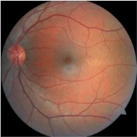
Original Image


blurred_image = image.filter(ImageFilter.BoxBlur(radius = 1))
blurred_image          # blurred image 
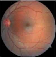
Blurred Image


PIL also provides another blurring filter GaussianBlur, which can be also applied to images to apply blurring effect on images. 
PIL.ImageFilter.GaussianBlur(radius = 2)

Sharpening 

A sharpening filter is an image filter that intensifies the edges and intricate features in a picture, making them more distinct and visually captivating. The main objective of sharpening is to enhance the clarity and sharpness of a picture. Multiple sharpening strategies exist, and a prevalent one involves using convolution processes with a designated kernel or filter.

In the field of image processing, a kernel refers to a compact matrix that is applied to the picture using convolution. This method allows for various operations such as blurring, sharpening, or detecting edges. The sharpening filter often employs a kernel that highlights the disparities in brightness among adjacent pixels, intensifying transitions and edges.

PIL.ImageFilter.Kernel(size, kernel, scale = None, offset = 0)
Create a convolution kernel. The present iteration only accommodates integer and floating-point kernels of dimensions 3x3 and 5x5. Currently, kernels may only be used on photos that are in the "L" and "RGB" formats.
PARAMETERS
  • size – Kernel size, given as (width, height). In the current version, this must be (3,3) or (5,5).
  • kernel – A sequence containing kernel weights. The kernel will be flipped vertically before being applied to the image.
  • scale – Scale factor. If given, the result for each pixel is divided by this value. The default is the sum of the kernel weights.
  • offset – Offset. If given, this value is added to the result, after it has been divided by the scale factor.
Code Example:
from PIL import Image
from PIL import ImageFilter
image = Image.open("drd.jpg")
image          # original image without blur filter
Original Image


# Define a kernal as a list of coefficients
kernel = [-1, -1, -1, -1, 9, -1, -1, -1, -1]   # For a 3x3 kernel with a central weight of 9
sharpened_image = image.filter(ImageFilter.kernel((3,3), kernel, scale = 1, offset = 0))
sharpened_image
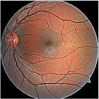
Sharpened Image


PIL also support filter such as Unsharmask for image processing. 
class PIL.ImageFilter.UnsharpMask(radius = 2, percent = 150, threshold = 3)
This is Unsharp mask filter.
PARAMETERS

  • radius – Blur Radius
  • percent – Unsharp strength, in percent
  • threshold – Threshold controls the minimum brightness change that will be sharpened.

Rank Filter

A rank filter is an image filter that applies a pixel-wise operation using the pixel values in the surrounding area of each pixel. Rank filters differ from linear filters in that they take into account the order or rank of pixel values in the neighborhood, rather than using a weighted average of pixel values. The main concept is to substitute the center pixel with the pixel value that corresponds to a certain rank, such as the lowest, highest, or middle value, within the nearby area.

Min Filter

class PIL.ImageFilter.MinFilter(size = 3)
Creates a min filter, which picks the lowest pixel value in a window with the given size.
where, size - The kernel size, in pixels.
Code Example:
min_image = image.filter(ImageFilter.MinFilter(size = 3))
min_image

Median Filter

class PIL.ImageFilter.MedianFilter(size =3)
Creates a median filter, which picks the meadian pixel value in a window with the given size.
where, size - The kernel size, in pixels.
Code Example:
median_image = image.filter(ImageFilter.MedianFilter(size = 3)
median_image

Max Filter

class PIL.ImageFilter.MinFilter(size = 3)
Creates a max filter, which picks the largest pixel value in a window with the given size.
where, size - The kernel size, in pixels.
Code Example:
max_image = image.filter(ImageFilter.MaxFilter(size = 3)
max_image

Mode Filter

class PIL.ImageFilter.ModeFilter(size = 3)
Develop a mode filter. Determines the pixel value that appears most often inside a box of the specified dimensions. Pixel values that have a frequency of one or two are disregarded; if no pixel value has a frequency greater than two, the original pixel value is retained.
Code Example:
mode_image = image.filter(ImageFilter.ModeFilter(size = 3)
mode_image
Rank Filter

That's it for Image Module and ImageFilter Module of PIL python library for Image handling and Image processing, I will write in more detail about ImageEnhance Module in another post. 
Keep in touch and Good Luck!

Thursday, January 4, 2024

How Computer See an Image


Did you ever image how a computer sees an image. Well thinking of image from the computer perspective image is nothing but the matrix of number, in which each cell of matrix identified as pixel and the value of pixel define a color combination or intensity of light.

Image as Function

An image can be expressed as a mathematical function that depends on two variables, x and y, which specify a two-dimensional region. A digital picture consists of a matrix of pixels. A pixel is the fundamental unit of a picture. An image is composed of pixels, each with a value that represents the intensity of light at a specific location within the image. Now, let's examine an example image, after implementing the pixel grid onto it.


The image seen above has dimensions of 28 × 28. The dimensions of the picture are 28 pixels in width and 28 pixels in height. Therefore, the total number of pixels is 784, which is calculated by multiplying 28 by 28. Given an image with dimensions of 224 × 250, the matrix representing the picture will have a dimensionality of (224, 250). Each element in the matrix corresponds to a pixel and indicates the brightness intensity of that pixel. The value of zero corresponds to the color black, whereas the value of 255 corresponds to the color white.

Color Images

Grayscale pictures assign a single-color intensity value to each pixel, whereas color images in the RGB system consist of three channels (red, green, and blue). To clarify, color pictures are encoded using three matrices: one matrix represents the red intensity of each pixel, another matrix represents the green intensity, and the third matrix represents the blue intensity.

RGB Channels of Colored Image

Image Processing

During machine learning (ML) projects, it is customary to do a data pretreatment or cleaning phase. As a machine learning engineer, a significant portion of your work will be dedicated to data preprocessing and data preparation prior to constructing your learning model. The objective of this stage is to prepare your data for the machine learning model, facilitating its analysis and computer processing. This statement also applies to images. To effectively address the issue at hand and use the available dataset, it is necessary to do data preprocessing before inputting the photos into the machine learning model.
Image processing includes basic operations such as imagine scaling. The pre-processing responsibilities include many operations such as geometric and color transformations, converting color images to grayscale, and more.  The obtained data is often disorganized and originates from several sources. 

Converting Color Image to Grayscale Image


Data Augmentation

Another prevalent preprocessing approach is enhancing the current dataset by adding altered copies of the original images. Scaling, rotations, and other affine transformations are often used to increase the size of your dataset and expose the neural network to a diverse range of picture variants. This enhances the probability of your model accurately identifying items regardless of their appearance or configuration.

Feature Extraction

Feature extraction is an essential element of the computer vision process. The DL model revolves on the concept of extracting valuable characteristics that accurately delineate the objects in the picture.
In the context of machine learning, a feature refers to a quantifiable attribute or characteristic of an observed phenomena. Features are the data inputs that are provided to a machine learning model in order to generate a prediction or classification. Assume you want to forecast the cost of a home. The input characteristics, such as the area, number of rooms, and bathrooms, will be used by the model to get a forecasted price. Choosing effective attributes that distinctly differentiate your items enhances the prediction capability of machine learning algorithms.

I will write more in detail about Data Augmentation and Feature Extraction for Image Classification using Deep Learning in Python programming language, stay tune!
Here is the link of my notebook for the above amusing results: Computer Vision - Practical Approach | Kaggle